
Only a little while ago we added Mistral AI’s Timestral-123M forecasting model to Carla (1). Things move fast: on November 12, 2026, Continuous Intelligence introduced ci-proto, a zero-shot forecasting foundation model built on Mamba-3 state-space blocks instead of Transformers (2). Because our current priority is building out Carla’s client-side model zoo, we took on the challenge of bringing ci-proto into the browser on stock WebGPU and ONNX.
In the November 13, 2026 AutoGluon fev-bench snapshot across 100 tasks, ci-proto ranks #1 on the 35-model default public view (90.00% SQL win rate, 51.51 skill score) and #3 across all 52 evaluated methods (84.37% SQL win rate, ahead of Timestral-123M at #5 with 81.06%) (3). Adding it to the same local browser runtime required three engineering steps: translating Mamba-3’s recurrent state-space scan into loop-free ONNX, porting reference-compatible float64 calendar and differencing logic to Rust and WebAssembly, and reducing multivariate GPU memory enough to run reliably on ordinary laptops.
Interactive demo
The interactive widget below starts with Timestral-5M (12 MB) so nothing large downloads on page load. You can switch the model selector to ci-proto (~346 MB) inside this article to run our packaged WebGPU runtime on your device.
Try this quick comparison to see the host pipeline and VariateMixer at work:
- Switch the model selector to ci-proto (~346 MB) and select the Orders (Rohlik) or Sales (Rossmann) tab.
- Click Download & run ci-proto (~346 MB) and watch the status header step from the univariate fast path (
~288 MiB GPU) into loading the+21.8 MBmultivariate covariate graph when covariates are active. - Toggle the covariate checkboxes on and off below the chart (on Orders,
ci-protoachieved 84.0% lower quantile loss vs. running without covariates in our headless Chrome check), or switch back to Timestral-5M on the same horizon slider to compare predictions side by side.
Download warning: Selecting
ci-protodownloads~346 MBon first use (335.6 MBshared FP16 external weights plus the10.1 MBunivariate ONNX graph; enabling covariates lazily fetches an extra21.8 MBmultivariate graph) and stores the files in browser cache. Desktop Chrome or Edge with WebGPU is recommended.
Uses ci-proto, released by Continuous Intelligence. Continuous Intelligence does not endorse or approve this product or service.
You can also test ci-proto directly on live Parquet slices across all of Carla’s forecasting dataset pages (such as Rohlik grocery orders, Nord Pool electricity prices, and Rossmann store sales); once cached here, those pages reuse the same browser weights without re-downloading. For full benchmark context, explore the 100-task Timestral-123M vs. ci-proto head-to-head breakdown or the time series benchmark suite.
What makes ci-proto different from Timestral?
Both ci-proto and Timestral-123M target zero-shot probabilistic forecasting with past and known covariates, yet they take opposite architectural routes (1,2).
In Continuous Intelligence’s announcement, ci-proto pairs a state space sequence mixer with cross-variate attention instead of a standard causal Transformer stack, highlighting “64× the context window of others” (relative to common 512-step baselines, i.e., 32,768 steps = 64×, and extending up to 2M+ steps in Continuous Intelligence’s separate upstream Python model-long.ckpt checkpoint) so forecasts absorb multi-year history without truncating seasonal cycles. Its model.ckpt checkpoint contains 167.2M unique parameters across 16 blocks after deduplicating weight-tied bidirectional state space cells (218.5M entries before tying); our browser WebGPU v1 runtime ports model.ckpt, which covers contexts up to 16,384 steps (32× a 512-step baseline).
| Dimension | Timestral-123M (Carla Engine) | ci-proto (model.ckpt WebGPU v1) |
|---|---|---|
| Organization | Mistral AI | Continuous Intelligence |
| Sequence backbone | 20 causal Transformer blocks (DHF, RoPE) | 16 weight-tied Mamba-3 SSD blocks + VariateMixer |
| Parameters | 122.6M | 167.2M unique (218.5M untied state_dict) |
| fev-bench (Nov 13, 2026, 52-model pool) | 81.06% SQL win rate (#5; skill 50.18) | 84.37% SQL win rate (#3; skill 51.51) |
| fev-bench (Nov 13, 2026, 35-model public view) | Not listed (Timestral-209M at #3: 87.06%) | 90.00% SQL win rate (#1; skill 51.51) |
| Context range ported | Up to 32,768 steps (patch 32) | Up to 16,384 steps in v1 (patch 32) |
| Predictive quantiles | 21 quantiles (P01 through P99) | 9 calibrated quantiles (P10 through P90) |
| Test-time augmentation | Optional sign-flip symmetry | Trend/running-total differencing, calendar channels, sign-flip TTA, band calibration |
| FP16 ONNX download | ~246 MB single graph | 335.6 MB shared .onnx.data + 10.1 MB univ / 21.8 MB mv |
| Licence | Apache-2.0 | ci-proto Code and Model Licence v1.0 |
Leaderboard note: Both columns compare models on the November 13, 2026
fev-benchsnapshot (100tasks, autogluon/fev) (3). Win rates depend on the pairwise model pool (52total evaluated models vs. the35-model default public subset, whereTimestral-209Mrepresents the Timestral family), while SQL skill scores (51.51vs.50.18) stay constant across views.
For task-by-task Scaled Quantile Loss (SQL) breakdowns across all 100 tasks, see Carla’s head-to-head empirical benchmark tables:
ci-protovs.TimeH2O-v1(50–50split;#1vs.#2on the 35-model public view)ci-protovs.Timestral-209M(55–45win record against Mistral’s largest public checkpoint)ci-protovs.Timestral-123M(53–47win record against Carla’s Google Sheets engine)ci-protovs.t0-gamma(69–31win record)ci-protovs.TimesFM-3(78–22win record vs. Google’s foundation model)
For spreadsheet users, those differences come down to three practical trade-offs:
- Calendar & cumulative awareness:
ci-protoadds automatic trend/running-total differencing, holiday channels, and band calibration in the host pipeline, helping on retail orders and daily business schedules. - Long multi-year horizons: Both architectures look far past
512-step baselines without truncating seasonal cycles. - Zero-server privacy: Both execute 100% locally on WebGPU, keeping revenue and staffing tables in the browser.
Which model should I pick?
- Timestral-123M (
~246 MB): Faster cold load, ultra-long hourly histories (32,768steps), and extreme tail quantiles (P01–P99). - ci-proto (
~346 MB): Top-ranked in the default publicfev-benchview, with strong covariate support, automatic cumulative/trend differencing, and cross-series (VariateMixer) sensitivity on daily and weekly business tables.
How do we run Mamba-3 in stock WebGPU without custom kernels?
Recurrent state space loops are awkward to export cleanly into browser ONNX graphs. Rather than building a custom C++ operator fork or hand-writing custom WGSL shaders for every Mamba-3 variant, we decomposed Mamba3Reference’s trapezoidal + MIMO (rank = 4, 20 heads, headdim = 64, d_state = 128, non-interleaved RoPE, zero causal conv) recurrence algebraically into pure loop-free tensor ops.
Each sequence splits into fixed chunk_size = 16 chunks: for v1’s 16,384-step maximum context (522 patch tokens including the 320-step output window), forward passes use up to 33 active chunks (ceil(522 / 16)), sliced from a precomputed 64 × 64 causal mask buffer (supporting up to 1,024 patches). Inside every block, execution proceeds in three stages built from matrix multiplications (MatMul) and elementwise tensor operations (Exp, CumSum, Where, scaling) natively supported by stock onnxruntime-web 1.31.1 on WebGPU (4):
- Intra-chunk blocks: Lower-triangular
MatMulplus elementwise exponential decay (segsum+Exp+Where) computes within-chunk interactions without sequential loops. - Cross-chunk boundary coupling: Each chunk summarizes its terminal boundary state into fixed-size accumulators via one fused
emit_stateMatMul. - Inter-chunk parallel scan:
CumSum, exponential masking, and ann_chunks × n_chunksMatMulpropagate state across chunks in one pass.
Two numerical rules keep parity intact. First, normalization reductions, time-step discretization (A, DT), cumulative RoPE angles, intra-chunk and inter-chunk decay factors, and state accumulation stay in FP32. Only 2D linear projection matrices (>= 4096 elements) use FP16 storage inside ci_proto_fp16w.onnx.data. Second, because VariateMixer is strictly bypassed when channels == 1, we export two slim ONNX graph headers sharing that single 335.6 MB external weight binary via ORT externalData: ci_proto_univ_fp16w.onnx (10.1 MB) for univariate forecasting and ci_proto_mv_fp16w.onnx (21.8 MB) for multivariate covariates and cohorts. While both graphs share one downloaded 335.6 MB (~320.1 MiB) external-data binary at the network and JavaScript buffer level, ONNX Runtime still allocates separate GPU-resident weight buffers for each initialized session (287.70 MiB for univ and 637.78 MiB for mv). Throughout this report, download sizes use decimal megabytes (MB) and GPU or process memory probes use binary mebibytes (MiB).
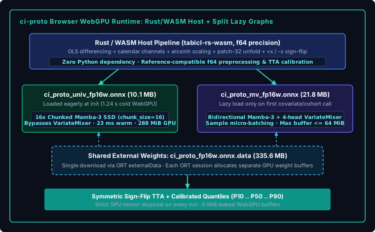
All preprocessing and postprocessing run inside tabicl-rs-wasm in f64 precision matching the upstream Python host pipeline. On bike_sharing_h24, the end-to-end Rust/WASM plus WebGPU fp16w pipeline matches PyTorch FP32 within an integer-rounded max_abs = 1 difference. On rohlik_orders_1d_brno and rossmann_1d_cohort8, browser WebGPU matches PyTorch FP32 within 0.027% and 0.007% relative SQL difference.
Why did browser GPU memory spike, and how did we cut it by 61%?
While single-series (univ-only) inference ran comfortably in ~288 MiB of live GPU buffers, profiling the isolated multivariate (mv-only) graph on Apple Metal WebGPU exposed two real browser memory blockers: peak intermediate GPU buffer allocations reached 4,949.1 MiB (5,275.5 MiB when paired eagerly with the univariate graph), and a single storage buffer hit 180.0 MiB, exceeding Chromium’s 128 MiB maxStorageBufferBindingSize limit.
Three targeted fixes solved the multivariate bottleneck:
- Eliminated GPU-to-CPU fallback breaks: Replaced
torch.splitprojections (which emitted CPU-onlySplitToSequenceandSequenceAtnodes) with explicitSliceops, and replaced dynamic boolean indexing around reverse state selection (which emittedNonZeroandScatterND) with sequential bidirectional scans blended by maskedWhereops. Separately, earlier graph cleanups rewroteEinsumnodes into broadcastMul/sum/MatMul, loweredPow(x, 2)toMul(x, x), and resolvedCastLikeinto explicitCastso all profiled floating-point model operations execute onWebGpuExecutionProvider(leaving only scalarint64shape and control ops on CPU). - Narrowed chunk size (
32 -> 16): Halved 5D intermediate Mamba-3 chunk tensors (max_chunks = 64mask ceiling; up to33active chunks for522v1 patches). - Sample micro-batching on WebGPU: Because Mamba-3
TimeMixerandVariateMixerhave zero dependencies across axis 0 (samples), looping over sign-flip+x/-xviews one sample at a time on GPU keeps intermediates strictly bounded.
Peak mv-only WebGPU buffer memory dropped by 61.4% (4,949.1 MiB -> 1,909.1 MiB), cumulative GPU buffer churn across 4 MV runs fell by 81.6% (20,267.4 MiB -> 3,730.9 MiB), and maximum single GPU buffer allocation fell by 2.81× from 180.0 MiB down to 64.00 MiB, half of Chrome’s 128 MiB storage binding ceiling. In the isolated probes, all tracked GPUBuffer objects are explicitly destroyed (0 MiB live tracked GPU buffers after dispose(), destroyCalls === createCalls). Under macOS unified memory, Chrome’s OS ps RSS drops partially rather than immediately returning to baseline (4,382.1 MiB -> 3,861.9 MiB total across browser processes; 482.6 MiB -> 224.2 MiB in the GPU process).
How does lazy multivariate loading cut cold startup by 74%?
Because ORT builds separate GPU weight allocations per session even when sharing .onnx.data, eager initialization compiled both ONNX graphs upfront (287.70 MiB GPU weights for univ + 637.78 MiB for mv = 925.49 MiB live idle GPU buffers, taking 4.72 seconds in Chrome before running a single forecast). Univariate users paid the multivariate graph’s initialization latency and VRAM cost without ever calling VariateMixer.
Changing createCiProtoForecaster() to lazyMvSession = true by default fixed both:
- Eager univariate probe: On init, Carla fetches and compiles only
ci_proto_univ_fp16w.onnxplus the shared335.6 MB.onnx.datafile. That still validates WebGPU adapter health and triggers WASM fallback immediately if needed. - Single-flight lazy
mvSession: Fetchingci_proto_mv_fp16w.onnxand callingInferenceSession.createhappens on demand on the first covariate or cohort forecast, reusing the already-fetched CPU.onnx.dataArrayBufferwithout re-downloading while ORT uploadsmv’s separate637.78 MiBGPU weight allocations once needed. - Univariate fast path: Users forecasting a single target series keep
mvSessionLoaded === falsefor the entire session, saving~638 MiBof GPU weight allocations and~3.5 secondsof shader compilation.
Verified in Google Chrome for Testing 157.0.8103.78 running the packaged MV3 extension worker under Apple Metal-3 WebGPU:
| Benchmark Metric | Eager Paired Load | Lazy MV (lazyMvSession = true) | Change |
|---|---|---|---|
Chrome cold init (sessionCreateMs) | 4,724.6 ms | 1,238.1 ms | -73.8% |
Isolated probe afterLoad live GPU | 925.49 MiB (708 buffers) | 287.70 MiB (281 buffers) | -68.9% |
Isolated probe afterLoad OS ps RSS | 2,507.0 MiB | 1,844.9 MiB | -26.4% |
Warm bike_sharing_h24 (univ) | 22.9–23.4 ms | 23.0–23.2 ms (mvSessionLoaded = false) | Even; zero MV overhead |
First MV (rohlik_orders_1d_brno) | 1,067.5 ms | 4,574.3 ms (3,493.4 ms lazy MV init + 1,056.1 ms warm) | Paid once on MV demand |
8-series cohort (rossmann_1d_cohort8) | 3,457.8 ms | 3,460.0 ms (0.007% SQL delta) | Parity preserved |
Just as our Kumo Tabular browser port uses GPU-resident context caches and bounded tiles to make large tabular workloads fit inside consumer laptop memory, split-graph lazy loading keeps browser WebGPU sessions fast for simple tasks without giving up full multivariate accuracy when covariates arrive.
What’s next for Carla?
ci-proto is the next addition to Carla’s local time-series model zoo, joining Timestral-123M for zero-shot forecasting directly inside Google Sheets. Single-series forecasts stay fast on a laptop GPU (~23 ms warm after load). Multi-series cohorts with holidays and covariates take a few seconds, still running locally without a backend prediction server. The broader lesson mirrors our browser port of Kumo Tabular: running a frontier foundation model on user hardware requires faithful host math, compatible GPU operators, and disciplined memory bounds, not just an ONNX export.
Growing Carla’s local model zoo gives spreadsheet users real choice within the same forecasting task. Teams can compare ci-proto against Timestral-123M on our time series benchmarks, then weigh forecast accuracy, interval calibration, download footprint, and local speed for their own sheet and device. Carla can recommend a default while leaving the model choice and its assumptions visible.
Install the Carla Chrome extension to run local forecasting in Google Sheets with Timestral-123M today, or test ci-proto directly in this browser tab using the interactive demo above as final cross-platform Chrome validation wraps up.
